3/12/2020
An Analysis of Speeding
As part of a larger project I wanted to see at what speed over a speed limit are drivers more likely to be pulled over by police. The only traffic violation data I could find that actually included data about the speed versus the speed limit was a dataset from Montgomery County, Maryland.
Cleaning the Data
I accessed the data through an online data viewer to begin with. I wanted to reduce the data as much as I could because I didn’t need all of the 1.6 million traffic violations from Montgomery County from 2015 until now, just the speeding violations. I looked at the descriptions of the violations and correlated them with their charge number. Through this I found the following charge codes which relate to speeding:
- 21-801(a)
- 21-801(b)
- 21-801(c)
- 21-801(d)
- 21-801(e)
- 21-801(f)
- 21-801(g)
- 21-801(h)
- 21-801-1
Filtering for these reduced the dataset from ~1.6 million to 258,280. I downloaded the dataset as a csv file and opened it in Excel. The dataset contained 43 columns of data. I removed the ones I didn’t need in Excel and ended up with 16 columns.
I had a couple decisions to make which related to the core reasons for looking at these numbers:
- Should I include speeding that resulted in an accident? (10,098 datapoints)
- Should I include speeding that resulted from an impaired driver (DUI)? (52 datapoints, 15 of those overlapped with accidents)
Because the intent of this project was to determine the speed at which a normal person is likelier to be pulled over I thought it would be good to exclude events in which a person’s speed was recorded only because they were exceeding the speed limit and nothing else. It is possible that some stops which were originally for speeding later turned into DUIs, but I decided that I could afford to exclude the group as a whole without sacrificing too many datapoints. All speeding violations that resulted in an accident were good to be excluded because it is not evident that the person would have been stopped if not for the accident. After removing accident and alcohol related violations I was left with 248,145 datapoints.
The core information I was interested in was the information in the “Description” column in which some variation of the following was written: EXCEEDED POSTED SPEED LIMIT: 55 IN A 25. Some descriptions were less descriptive and only said something like EXCEEDING THE POSTED SPEED LIMIT OF 30 MPH. I decided that in order to extract the numbers from the descriptions and clean away the text that did not include the violating speed I would import the data into Python and work from there. I used VS Code for all of the Python-powered data cleaning.
I read the csv and stripped everything but the numbers from the descriptions column (re.sub('\D', '', row[0])) and then appended the results to a list named nums. I noticed a pattern in the description where the violating speed was always listed first and the speed limit was listed second. I would validate this later, but my expectation was that the cleaned descriptions would yield 4 or 5 digit numbers with either the first 2 or 3 digits being the violating speed and the last two digits always being the speed limit.
import re
import csv
nums = []
with open('cTrafs.csv', 'r') as rfile:
  csvreader = csv.reader(rfile)
  for row in csvreader:
    nums.append(re.sub('\D', '', row[0]))
The nums list contained a bunch of strings of numbers. I wanted to see what the minimum and maximum values in the list of strings of numbers was. Because the min() and max() methods only work on integers I had to convert all of the strings of numbers into integers. I didn’t want to do this permanently, just to get the minimum and maximum.
ints = []
for k in nums:
  if k != '':
    ints.append(int(k))
What I found was concerning. The minimum was 0, and the maximum was 86606040. It was possible there was an error in text stripping and I felt that the best diagnostic at this point was to re-attach these numbers to the csv and compare the stripped descriptions to the actual descriptions. With the numbers back in the csv I opened Excel, sorted the numbers column by largest to smallest and found the culprit. Eight datapoints had irregular entries for the descriptions. Two of these contained two sets of numbers: *DRIVING VEHICLE IN EXCESS OF REASONABLE AND PRUDENT SPEED ON HIGHWAY 86/60, 60/40 *DRIVING VEHICLE IN EXCESS OF REASONABLE AND PRUDENT SPEED ON HIGHWAY 80-90 IN 55
The other 6 contained obviously incorrect numbers: *EXCEEDING MAXIMUM SPEED: 4940 MPH IN A POSTED 40 MPH ZONE *EXCEEDING MAXIMUM SPEED: 4940 MPH IN A POSTED 40 MPH ZONE *EXCEEDING MAXIMUM SPEED: 3930 MPH IN A POSTED 30 MPH ZONE *EXCEEDING MAXIMUM SPEED: 3930 MPH IN A POSTED 30 MPH ZONE *EXCEEDING MAXIMUM SPEED: 3930 MPH IN A POSTED 30 MPH ZONE *EXCEEDING POSTED MAXIMUM SPEED LIMIT: 330 MPH IN A POSTED 30 MPH ZONE

These 8 entries were deleted from the dataset and the Python script was re-run. This time the maximum number was 13955, which makes sense as the speed was 139 and the limit was 55.
The minimum of 0 was the same as previously, but doesn’t really matter because entries with values less than 4 digits long would be thrown out. The decision to throw out all numbers less than four digits was made because all speed limits (other than 5mph) are two digits long and a violating speed must be at least two digits long. There were only three instances in which a 5mph speed limit was violated and in each case the violating speed was so egregious that it wouldn’t be helpful to the analysis. Anecdotally, it seems that 5mph speed limit zones are quite uncommon and studying this range would not be useful anyway.
With the re-cleaned numbers it was time to split them up to get the violating speeds and the speed limits.
spd = []
lmt = []
for n in nums:
  if len(n) > 3:
    if len(n) == 5:
      spd.append(n[:3])
      lmt.append(n[3:])
    elif len(n) == 4:
      spd.append(n[:2])
      lmt.append(n[2:])
After separating out the speeds and speed limits and throwing away the numbers less than or equal to 3 digits long I ended up with 106,847 datapoints. I wrote the new columns to a new csv and combined that csv with the original csv in Excel.
full = zip(spd, lmt)
with open('full.csv', mode='w', newline='\n') as wfile:
  csvwriter = csv.writer(wfile, delimiter=',')
  csvwriter.writerow(['speed', 'speed_limit'])
  for k in full:
    csvwriter.writerow(k)
The final cleaning process involved checking to see if the number in the speed column was larger than the number in the speed limit column. I added a new column in Excel and added a formula to calculate the difference between the speed and speed limit. I then sorted the “Difference” column by smallest to largest and noted the negative values. There were 18 of these negative values and they were all removed to bring the dataset to 106,829. I also noticed, in Excel, that one of the speed limits was listed as “49”, which is likely to be a data entry error. That datapoint was removed to bring the datapoints to 106,828.
I noticed that a common trend in these negative values is that the number of the highway was used and that was the source of the error. I decided to then check the values in the “Description” column for any occurence of the word “Highway”. There were 4,217 datapoints with the word “Highway” in the description and from a cursory view most of them made sense to leave in the dataset. However I wanted to ensure that the data was as clean as possible and so I decided to make two datasets. One dataset with the “Highway” entries and one without. The dataset without contained 102,610 datapoints.
Analyzing the Data
My original intention for this project was to determine the speed at which a person is more likely to be pulled over at. Finding this out would give an idea of how fast a person can reasonably go without an expectation of being pulled over and ticketed. With over 100,000 datapoints I believed a reasonable estimation could be done, despite the fact that all of the data came from one location: Montogomery County, Maryland. In order to resolve my initial inquiry I decided that I would want to look at the most common speed at which people are pulled over for all speed limit zones and then look at the most common speed per speed limit zone.
The libraries I expected to use were:
- Pandas: I wanted to load the data into a Pandas data frame because it is much easier to analyze and manipulate the data this way. I also did basic data analysis with this package.
- Seaborn: I used the box plot and violin plot to visualize outliers and data spread.
- MatPlotLib: I used MatPlotLib to help create some of the visualizations.
import pandas as pd
import seaborn as sns
import matplotlib as mlab
import matplotlib.pyplot as plt
I opened up the aforementioned csv using the Pandas library in a Jupyter notebook. I viewed the head just to be sure the data was loaded in the dataframe correctly.
data = pd.read_csv('ctrafs_full.csv')
df = pd.Dataframe(data)
df.head()
I also used df.info() and df.describe() to check data types in the columns and get a quick statistical view of the dataset. I then made a boxplot of the speeds to see how widely the data was spread and to visualize the outliers.
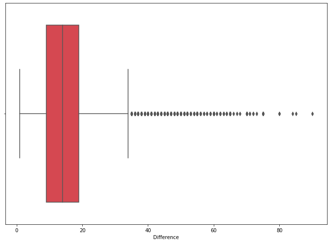
The mean, median, and mode for the difference at this point was 14.98, 14, and 9. In order to clean the data a little bit more I decided to remove the upper outliers and keep the lower ones. The upper outliers represent speeds which likely do not reflect normal driving. The bottom outliers would be kept because they represent speeding violations, despite the fact that they may be abnormally low. I calculated the upper quartile and then created a new dataframe which removes datapoints where the “Difference” exceeds the high value.
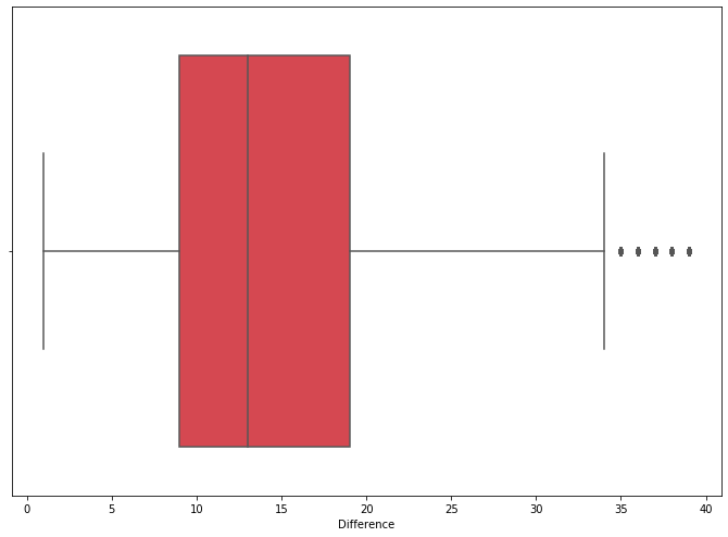
q_hi = df["Difference"].quantile(0.99)
n_df = df[(df["Difference"] < q_hi)]
The upper quantile was 40. Cutting the upper outliers resulted in 105,560 datapoints. The mean, median, and mode for the smaller dataset was 14.59, 13, and 9.
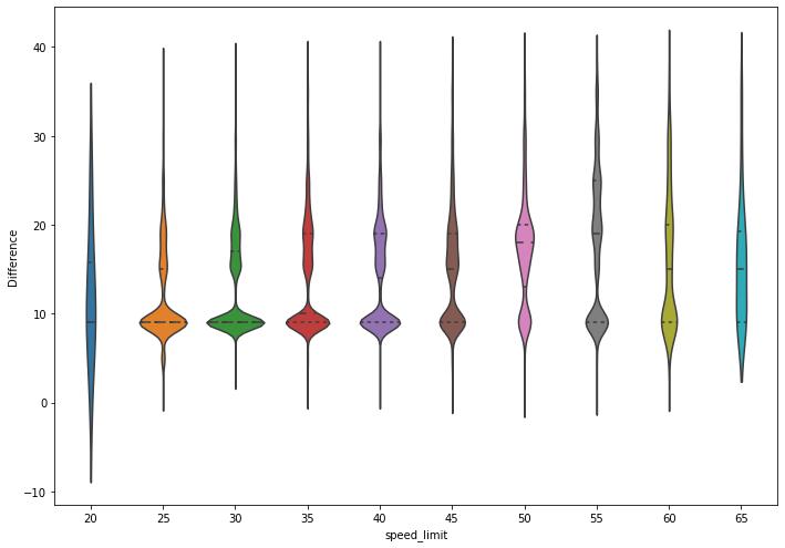
To get an idea of which speed over the limit is most common I ran the method .value_counts() on the “Difference” column and found that, by far, 9 mph was the most common. The second most common was 19 mph. The 9 mph value had 49,159 (46.6%) violations while the second-most (19 mph) had 7,356 (7.0%). I made a histogram and violin chart to see how the data were distributed.
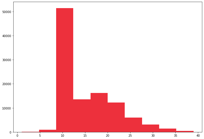
Initially it seemed quite odd that there was such a high concentration at 9 mph, but it makes sense if you consider that it appears police officers are willing to drop the actual reported mile down to save the driver some money and points. Looking at the Maryland Speeding Laws it seems quite clear that is what is happening here. Exceeding a posted speed limit by 1 to 9 mph gets you a $80 fine and one point whereas exceeding by 10 to 19 gets you a $90 fine and two points. Since it is likely that the 9 and 19 datapoints were artificially high not a lot of data can be determined from them. It could be assumed, however, that most traffic stops occur at least 9 mph over the speed limit, however. After 9 mph the next single-digit number with the most violations was 5 with only 606 violations, which is only 0.6% of all of the violations. The least ticketed was 2 mph over with just 4 violations.
To get a more granular look I broke up the dataframe into separate dataframes for each speed limit. I used n_df["speed_limit"].unique() to see a list of the unique speed limits. From there I made the datasets.
sl_20 = n_df.loc[df['speed_limit'] == 20]
sl_25 = n_df.loc[df['speed_limit'] == 25]
sl_30 = n_df.loc[df['speed_limit'] == 30]
sl_35 = n_df.loc[df['speed_limit'] == 35]
sl_40 = n_df.loc[df['speed_limit'] == 40]
sl_45 = n_df.loc[df['speed_limit'] == 45]
sl_50 = n_df.loc[df['speed_limit'] == 50]
sl_55 = n_df.loc[df['speed_limit'] == 55]
sl_60 = n_df.loc[df['speed_limit'] == 60]
sl_65 = n_df.loc[df['speed_limit'] == 65]
After this I used the .describe() method to evaluate the smaller datasets. The 20 mph dataset only contained 8 datapoints and so it was ignored. The 25 mph contained 5,273 datapoints and a similar distribution of violations.
| Speed over Limit | Number of Violations |
|---|---|
| 9 | 3,186 |
| 15 | 348 |
| 19 | 206 |
| 5 | 204 |
| 16 | 179 |
| … | … |
| 7 | 2 |
| 36 | 1 |
| 1 | 1 |
Similarly to the overall data the 25 mph speed limit breakdown shows a high incidence of violations at 9 mph (presumuably 9 mph +). The major difference in this speed limit versus the larger dataset is that 5 mph over is the fourth highest speed in terms of number of violations. Jumping to the 30 mph speed limit you can see that the 5 mph violation is significantly less common. The violin chart displays the difference quite well.
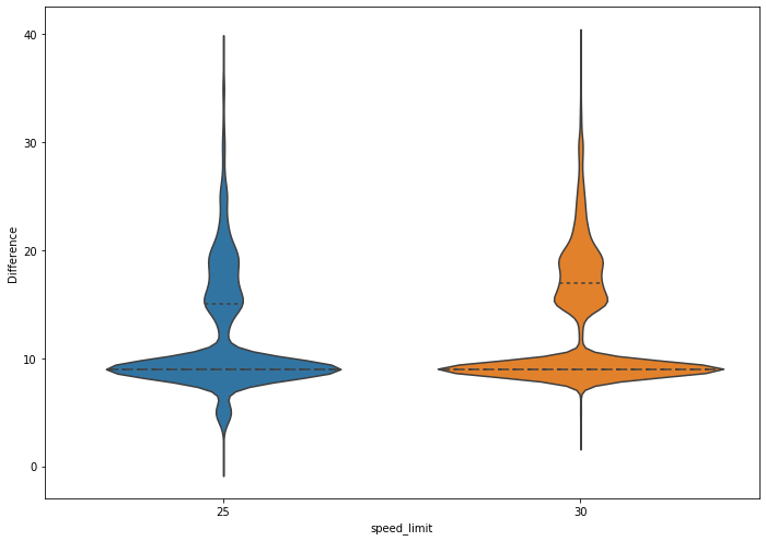
The trend of 9 mph and double-digit violations being far more popular follow in every other speed limit bracket and it is always 5 mph that is the 2nd most popular violation speed.
Conclusion
It is quite clear that in speed limit zones from 30mph and up going 9 mph or more over the speed limit will result in a speeding ticket more often than going 8 mph or less over the speed limit. In 25 mph or less speed limit zones there is less tolerance for speed over the limit. It would appear that, if you’re going to speed, keep it at 8 mph or less over the speed limit in speed limit zones above 25 mph to lower your risk of getting a ticket. That isn’t necessarily a recommendation, however. Speed limits are there for a reason and staying at or below the speed limit is likely to be the best chance at arriving at your destination safely.
The problem with this data is that it is all from one location. A broader dataset would show if the trends noticed here are local or if they do indeed represent a larger population. Unfortunately it does not appear that these datasets are widely available. So, this is as good of an analysis that can be done for now.
A future project will use the data gathered here to look at the optimal speed to travel in order to save the most money.
Anthony Miller
Software engineer